Transformation functions [wrangle]

(Builds on: Manipulation basics)

summarise() and mutate() work at the data frame level: they take a data frame as input and return a data frame as output. You combine these data frame functions with with vector functions: functions that take a vector as input and return a vector as output. The length of the output determines whether a given function work with summarise() or mutate():

summarise() works with summary functions; functions that take n inputs and return 1 output. This includes functions like sum() and mean() for numeric vectors; all() and any() for logical vectors; and str_c() with collapse for character vectors.
mutate() works with transformation functions: functions that take n inputs and return n outputs. So far you’ve mainly used vectorised maps, like - and +, or & and |. In this unit, you’ll learn some finer details of these functions, and learn a new class of functions called window functions.

library(tidyverse)

Vectorised map functions

Unary

The simplest type of transformation function is the “unary vectorised map”. This is a precise, but complicated name. Let’s unpack it and explain each component:

Unary means that the function takes a single vector as input.
Vectorised means that the function takes a vector as input and returns a vector of the same length as the output (but possibly a different type).
Map is a mathematical term that means that you can independently compute each element of the output from the corresponding piece of the input. In other words, if your input is x and your output is z, the only value of x that z[i] depends on is x[i].

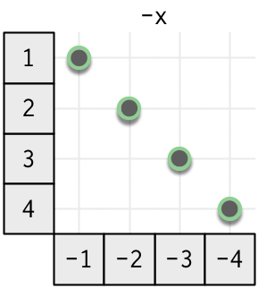
The diagram below shows a vectorised function, focusing on how the input is connected to the output. The input is on the left, and the output is on the bottom. You can see how each input affects the output by following the lines right and down; you can see how an output is computed from the input by following the lines up and left. The connections for a vectorised function are simple: each input only affects the output at the same position.

It’s helpful to organise unary vectorised maps by the type of input vector:

Numeric: most of these come from base R and include functions like log() and abs(), and operators like ! and -.

x1 <- c(1, 4, 2)
-x1
#> [1] -1 -4 -2

x2 <- c(TRUE, FALSE, FALSE)
!x2
#> [1] FALSE  TRUE  TRUE

Character: these are provided by stringr and include functions like str_length(), str_lower() and str_upper().
Date times: these are provided by lubridate and include functions like yday() and year().

Binary

Another extremely common class of transformation functions are the binary vectorised maps. These are similar to the unary transformation functions except that they take 2 vector inputs. You’ve used many of these functions already because they include the mathematical operators -, +, /, *, %% and %/%.

There is a new wrinkle with these functions: since they take two vectors, what happens if they are different lengths? For example, in x * 2 below, x has length 10, but y has length 1.

x <- sample(100, 10)
y <- 2

x * y
#>  [1]  18 166 118  32   2  90  94  54 136 142

R has a special set of rules that cover this situation called the recycling rules. Whenever you call a binary vectorised fuction with inputs of different lengths, R will recycle the shorter vector to be the same length as the longer. This is particularly useful when combined with summary operators:

x - min(x)
#>  [1]  8 82 58 15  0 44 46 26 67 70
(x - mean(x)) / sd(x)
#>  [1] -1.1889  1.4295  0.5803 -0.9412 -1.4720  0.0849  0.1557 -0.5520
#>  [9]  0.8987  1.0049

(You can use recycling rules with vectors that are not of length 1, but that makes it easy to write confusing code, so I don’t recommend it.)

Vectorised window functions

Vectorised map functions can be generalised to vectorised window functions. In a window function the output now depends on a contiguous window of values (i.e. a sequence with no gaps). Map functions are a special case of window functions because in a map function, the “window” is just a single value.

Offset

The simplest type of window is an offset. Each output value still depends on only a single input value, but the input and output are no longer aligned. The following diagram illustrates offsets in either direction.

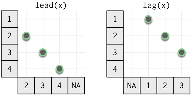
In dplyr you can use lead() (positive) and lag() (negative) to look at offsets.

tibble(
  x = 1:5,
  pos = lead(x),
  neg = lag(x)
)
#> # A tibble: 5 x 3
#>       x   pos   neg
#>   <int> <int> <int>
#> 1     1     2    NA
#> 2     2     3     1
#> 3     3     4     2
#> 4     4     5     3
#> 5     5    NA     4

Change the number of positions to look ahead or behind with the second argument, n.

Remember that these are vectorised functions, so the output must be the same length as the input. That means we need to pad either the beginning or the end of the vector. lead() and lag() pad with NA but you can change this value with the default argument.

lead() and lag() are very useful when combined with a binary vectorised map:

x == lag(x) tells you if x has changed compared to the previous value.
x - lag(x) tells you how x has changed.

Rolling

Rolling window functions are the next step up in complexity. Instead of a window of size one, they now have a fixed window of size m.

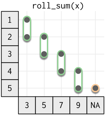
Neither base R not dplyr provide rolling functions, but you can get them from the RcppRoll package. By default the roll_ functions are not vectorised (they return shorter vectors), but you can make them vectorised by setting fill = NA.

library(RcppRoll)

tibble(
  x = 1:5,
  roll_sum = roll_sum(x, 2, fill = NA),
  roll_mean = roll_mean(x, 2, fill = NA)
)
#> # A tibble: 5 x 3
#>       x roll_sum roll_mean
#>   <int>    <dbl>     <dbl>
#> 1     1        3       1.5
#> 2     2        5       2.5
#> 3     3        7       3.5
#> 4     4        9       4.5
#> 5     5       NA        NA

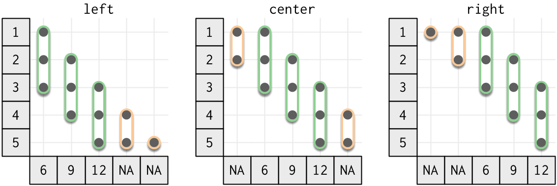
You can control how the window is aligned to the data with the align argument. The following figure shows n = 3 and the three possible values of align. Note that the output value is NA if there are less than 3 inputs.

Cumulative

The next step up in complexity are the cumulative functions, where the window size is no longer constant. A cumulative function uses all values up to the current position.

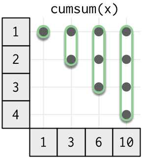
Base R includes the cumulative functions cumsum(), cumprod(), cummax(), and cummin(). dplyr provides a few others: cummean(), cumany(), cumall(). I’m not aware of any useful cumulative functions for strings or date/times.

library(RcppRoll)

tibble(
  x = 1:5,
  cumsum = cumsum(x),
  cummean = cummean(x)
)
#> # A tibble: 5 x 3
#>       x cumsum cummean
#>   <int>  <int>   <dbl>
#> 1     1      1     1.0
#> 2     2      3     1.5
#> 3     3      6     2.0
#> 4     4     10     2.5
#> 5     5     15     3.0

Complete

The most complex type of window function is the complete window function, where every output value depends on every input value.

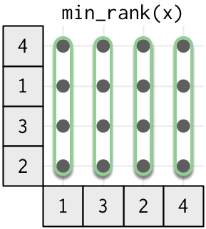
This class of window function includes all the ranking functions, because the rank of any value depends on the rank of all the other values. There are three key ranking functions that differ in how ties are handled:

tibble(
  x = c(10, 10, 10, 20, 20, 30),
  min = min_rank(x),
  dense = dense_rank(x),
  row_number = row_number(x)
)
#> # A tibble: 6 x 4
#>       x   min dense row_number
#>   <dbl> <int> <int>      <int>
#> 1    10     1     1          1
#> 2    10     1     1          2
#> 3    10     1     1          3
#> 4    20     4     2          4
#> 5    20     4     2          5
#> 6    30     6     3          6

Use desc() if you want the highest inputs to have the lowest ranks.

min_rank() works like sports ranking: if there are three people tied for first place, the next rank is 4th place. dense_rank() ensures that the ranks are “dense”, i.e. it doesn’t skip any ranks for ties. row_number() breaks ties so that every row gets a unique number. It’s easiest to understand the differences in terms of filtering:

min_rank(x) <= 2 will select all elements in first place, and will only select another if there wasn’t a tie for first.
dense_rank(x) <= 2 will select all elements tied for first place, and all elements tied for the next rank.
row_number(x) <= 2 will always select exactly two elements.

Ordering

So far we’ve dodged the question of what we mean by “before” and “after”, relying on the order of the rows. There are three ways to be more precise:

arrange() the data so you know exactly how the rows are ordered.
Use the order_by argument (if present), to order by a specific variable. This is more efficient than arrange() if you’re only computing a single window function.
Use the order_by() helper if there is no order_by argument.

The main difference between the arrange and order_by is what happens to the other columns:

df <- tribble(
  ~time, ~ value,
      7,       3,
      1,       5,
      5,       -2,
      3,       0
)

df %>% 
  arrange(time) %>%
  mutate(cumulate = cumsum(value))
#> # A tibble: 4 x 3
#>    time value cumulate
#>   <dbl> <dbl>    <dbl>
#> 1     1     5        5
#> 2     3     0        5
#> 3     5    -2        3
#> 4     7     3        6

df %>% 
  mutate(cumulate = order_by(time, cumsum(value)))
#> # A tibble: 4 x 3
#>    time value cumulate
#>   <dbl> <dbl>    <dbl>
#> 1     7     3        6
#> 2     1     5        5
#> 3     5    -2        3
#> 4     3     0        5